Boundary feedback control of the Korteweg-de Vries-Burgers' equation

We consider the Korteweg-de Vries-Burgers equation

$\displaystyle w_{t}-\varepsilon w_{xx}+\delta w_{xxx}+ww_{x}=0,\quad x\in [0,1],\quad t>0\, ,$ (1)

with $ \varepsilon $, $ \delta >0 $ and with some initial data

$\displaystyle w(x,0)=w_{0}(x),\quad x\in [0,1].$ (2)

In our paper we prove that the following nonlinear boundary control stabilizes (1)-(2)


$\displaystyle w\left( 0,t\right)$ $\displaystyle =$ $\displaystyle 0\, ,$ (3)
$\displaystyle w_{x}\left( 1,t\right)$ $\displaystyle =$ $\displaystyle -g_{1}\left( w\left( 1,t\right) \right)$  
  $\displaystyle \triangleq$ $\displaystyle -\frac{1}{\varepsilon }\left( c+\frac{1}{9c}w^{2}\left( 1,t\right) \right) w\left( 1,t\right) \, ,$ (4)
$\displaystyle w_{xx}\left( 1,t\right)$ $\displaystyle =$ $\displaystyle g_{2}\left( w\left( 1,t\right) \right)$  
  $\displaystyle \triangleq$ $\displaystyle \frac{1}{\varepsilon ^{2}}\left( c+\frac{1}{9c}w^{2}\left( 1,t)\right) \right) ^{2}w\left( 1,t\right) \, .$ (5)

It is clear that, since (4) and (5) are invertible functions, this control law can be implemented via any of the following three variables at the 1-boundary: $ \left( w_{x},w_{xx}\right) $, $ \left( w,w_{x}\right) $, $ \left( w,w_{xx}\right) $.
In order to formulate our problem as an abstract initial value problem we consider Hilbert spaces $ X=L^{2}(0,1) $, $ H=H^{1}(0,1) $, operator $ {\cal A}\, :\, \left( {\cal D}\left( {\cal A} \right) \subset X\right) \rightarrow X^{*} $ given by
$\displaystyle {\cal A}w=-\varepsilon w_{xx}+\delta w_{xxx}+\frac{1}{2}\left( w^{2}\right) _{x}\, ,$ (6)

and domain

$\displaystyle {\cal D}\left( {\cal A} \right) =\left\{ w\in H^{3}\left( 0,1\rig...
...\right) ,\, w''\left( 1\right) =g_{2}\left( w\left( 1\right) \right) \right\} .$

With the above notation our system (1), (2), (3)-(5) can be written in the form of

$\displaystyle \frac{dw}{dt}+{\cal A}w=0\, ,\qquad w\left( 0\right) =w_{0}\, .$ (7)

Our main result is formulated in the following theorem.

Theorem :   For any initial data $ w_{0}\in {\cal D}\left( {\cal A} \right) $ system (7) possesses a unique solution $ w\left( x,t\right) \in C\left( 0,\infty ;L^{2}\left( 0,1\right) \right) \cap C\left( 0,\infty ;H^{1}\left( 0,1\right) \right) $ with

  1. Global exponential stability in the $ L^{2} $-sense:

    $\displaystyle \left\Vert w\left( t\right) \right\Vert \leq \left\Vert w_{0} \right\Vert e^{-\varepsilon t},\qquad \forall t\geq 0\, ,$ (8)

  2. Global asymptotic and semi-global exponential stability in the $ H^{1} $-sense: there exist $ M>0 $ such that for any $ 0\leq \alpha <1 $

    $\displaystyle \left\Vert w\left( t\right) \right\Vert _{H^{1}}\leq \frac{M}{\sq...
...\right\Vert ^{2}_{H^{1}}}e^{-\alpha \varepsilon t}\, ,\quad \forall t\geq 0\, .$ (9)

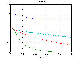
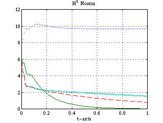
The proof can be found in our paper. Simulation Example

The following numerical simulation shows that our control law (3)-(5) achieves faster convergence than the control law

$\displaystyle w\left( 0,t\right)$ $\displaystyle =$ $\displaystyle 0\, ,$ (10)
$\displaystyle w_{x}\left( 1,t\right)$ $\displaystyle =$ $\displaystyle 0\, ,$ (11)
$\displaystyle w_{xx}\left( 1,t\right)$ $\displaystyle =$ $\displaystyle -\frac{1}{3\delta }w^{2}\left( 1,t\right) \, ,$ (12)

and an improved version of it
$\displaystyle w\left( 0,t\right)$ $\displaystyle =$ $\displaystyle 0\, ,$ (13)
$\displaystyle w_{x}\left( 1,t\right)$ $\displaystyle =$ $\displaystyle 0\, ,$ (14)
$\displaystyle w_{xx}\left( 1,t\right)$ $\displaystyle =$ $\displaystyle \frac{1}{\delta }\left( c+\frac{1}{9c}w^{2}\left( 1,t\right) \right) w\left( 1,t\right) \, ,\quad c>0\, .$ (15)

proposed by Liu and Krstic. A comparison is also made relative to the uncontrolled system consisting of the KdVB equation (1) and the boundary conditions

$\displaystyle w\left( 0,t\right) =0\, ,\quad w_{x}\left( 1,t\right) =w_{0}'\left( 1\right) \, ,\quad w_{xx}\left( 1,t\right) =w_{0}''\left( 1\right) \, .$ (16)

Click on the images to see animation!

Figure 1: KdVB equation: Comparison of Solutions
(a) Uncontrolled (b) Second Derivative Controlled (Quadratic)
(c) Second Derivative Controlled (Cubic) (d) Two Derivatives Controlled

Figure 2: Comparison of Norms. ... Uncontrolled, ooo Controlled Second Derivative (Quadratic),
- - - Controlled Second Derivative (Cubic), --- Two Derivatives Controlled


Maintained by Andras Balogh