![]()
![]()
![]()
![]()
![]()
![]()
![]()
![]()
![]()
Introduction
We stabilize the parabolic equilibrium profile in a 2D channel flow using actuators and sensors only at the wall. The control of channel flow was previously considered by Speyer and coworkers, and Bewley and coworkers, who derived feedback laws based on linear optimal control, and implemented by wall-normal actuation. With an objective to achieve global Lyapunov stabilization, we arrive at a feedback law using tangential actuation (using teamed pairs of synthetic jets or rotating disks) and only local measurements of wall shear stress, allowing to embed the feedback in MEMS hardware, without need for wiring. This feedback is shown to guarantee global stability in at least
The Equations with the Control
The channel flow can be described by the 2D Navier-Stokes equations
| (1) | |||
| (2) |
where
| (3) | |||
| (4) | |||
| (5) | |||
| (6) |
where k is a positive constant and
Numerical Simulation
The simulation example in this section, performed for Reynolds number
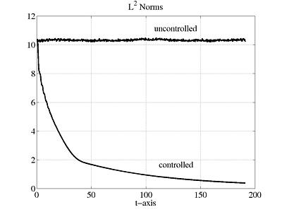
In Figure 1 we observe the stability enhancement resulting from the use of control.
It is expressed in terms of the ![]() -norm of the errors between the steady state
and the actual velocity field. (After the initial fast convergence the decay rate becomes very slow for large time in the controlled case. This behavior suggests the use
of state dependent high control gains which we consider a possible future topic.)
-norm of the errors between the steady state
and the actual velocity field. (After the initial fast convergence the decay rate becomes very slow for large time in the controlled case. This behavior suggests the use
of state dependent high control gains which we consider a possible future topic.)
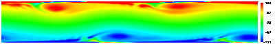
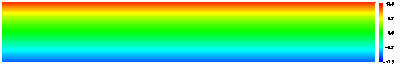
In the vorticity map, depicted in Figure 2 it is striking how uniform the vorticity field becomes for the controlled case, while we observe quasi-periodic bursting in the uncontrolled case. This figure (top), as well as those we obtained for other Reynolds numbers, agrees qualitatively with the vorticity maps obtained by Jimenez.
The uniformity of the wall shear stress
![]() in the controlled flow can be also observed in Figure 3.
in the controlled flow can be also observed in Figure 3.
|
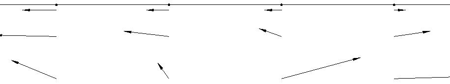
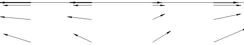
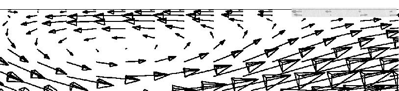
Our boundary feedback control (tangential actuation) adjusts the flow field near the upper boundary such that the controlled wall shear stress almost matches that of the steady state profile. The region is at the edge of a small recirculation bubble (Figure 4) of the uncontrolled flow, hence there are some flow vectors pointing in the upstream direction while others are oriented downstream. The time is relatively short (t=5) after the introduction of the control and the region is small. As a result it is still possible to see actuation both downstream and upstream. Nevertheles the controlled velocity varies continuously. Figure 4 shows that the effect of control is to smear the vortical structures out in the streamwise direction.
|
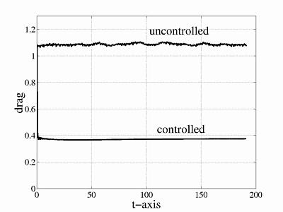
We obtain aproximately 60% drag reduction (Figure 5) as a byproduct of our special control law. The drag in the controlled case agrees with the drag corresponding to the laminar flow up to four decimal digits.